Overview of Neighbourhood Operations

index Introduction The Scanning Cell and its Neighbourhood How Neighbourhood Operations Work Statistical Neighbourhood Operations Sum Average Maximum Minimum Median Majority Minority Diversity Range Some Examples
Introduction Neighbourhood operations are a method of analysing data in a GIS environment. They are especially important when a situation requires the analysis of relationships between locations, rather than interpret the characteristics at individual locations. The Scanning Cell and its Neighbourhood Neighbourhood operations are commonly called ‘Focal Functions’ since each operation performed generates a value for the ‘focus’ of a neighbourhood. The neighbourhood focus is generally called the scanning cell and its neighbours – that is the cells surrounding it – are known as the scanning neighbourhood. The scanning neighbourhood can take on various sizes and shapes, which are defined by selecting the appropriate options in the GIS package. The most common neighbourhood shapes are:

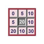
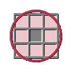
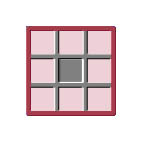
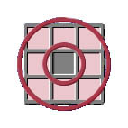
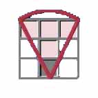
Note: in the above examples the scanning cell is shaded grey, and cells in the scanning neighbourhood (delimited by a red border) are shaded pink. Also note that the scanning neighbourhood for each of these neighbourhood shapes includes the scanning cell, with the exception of a donut shaped neighbourhood. You may notice that at this scale there appears to be no difference between the circular and square scanning neighbourhoods. In "Lesson 2 - Simple Interactive Examples", the difference between these scanning neighbourhood shapes is more evident. The GIS user can define any size for the neighbourhood, according to the problem at hand. The examples at the bottom of this page illustrate various instances where the different neighbourhood shapes may be used. How Neighbourhood Operations Work Neighbourhood operations work by moving across a raster grid map, one cell at a time. As each cell is visited, it becomes the scanning cell and a new value is computed for that cell as a function of its scanning neighbourhood. All computed values are then placed into the corresponding cells of the output map/theme.
Statistical Neighbourhood Operations Various statistics can be used to characterise the neighbourhood of a scanning cell. Note though, that as there are four general types of numerical data that can be present in an input map, the statistics which are used in the neighbourhood operations will depend on which data type is being studied (follow the links below to see information about each data type, including examples and the statistical operations that can be applied to such data): Ratio Interval Ordinal Nominal Note that if a function can be applied to data of any given type of the above, it can also be applied to the proceeding type. This module details nine statistical operations, namely Sum, Average, Maximum, Minimum, Median, Majority, Minority, Diversity and Range. An example scanning cell and its neighbourhood are shown below. Each statistical operation is then described along with its result for the example. Sum ( = 110) This operation adds the values of the scanning cell and its neighbours (i.e. the cells in its scanning neighbourhood), and stores this sum in the output theme. The input map data can be ratio or interval. An example of the use of SUM is to measure the density of features on a map, such as the generation of a residential density map encoded for the number of dwelling units per 100 hectares. Average ( = 12.22) This statistic calculates the mean value of the data present in the scanning neighbourhood. The input map data must be ratio or interval. AVERAGE is often used to "smooth" values in a map and as such is equivalent to a low pass filter in remote sensing. An example is the smoothing of terrain prior to analysis so as to remove small errors/noise in the data. Maximum ( = 30) The maximum operation returns the value of the cell in the scanning neighbourhood which has the highest value. The input map data can be ratio, interval or ordinal. An example of the use of this statistic is to value each cell according to the most valuable resource in the local area. Minimum ( = 0) This operation returns the value of the cell in the scanning neighbourhood with the lowest value. As with MAXIMUM, the input map data can be ratio, interval or ordinal. MINIMUM is often used to locate "pits" in an elevation map, with an example being its use in detecting "spurious pits" (single-cell depressions in elevation data) prior to runoff simulations. Median ( = 10) This operation returns the median (middle) value of the scanning neighbourhood values. The input map data may be ratio, interval or ordinal. The MEDIAN operation is used under similar circumstances to AVERAGE - ie. for smoothing values in a map. Majority ( = 10) This operation returns the value which occurs most frequently in the scanning neighbourhood. The input map data may be ratio, interval, ordinal or nominal. An example of the use of MAJORITY is to replace missing values in a map, such as assigning the most common land use in a neighbourhood to ‘data-less’ slivers or points on a digitised map. Minority ( = 30) The minority operation returns the value which occurs least frequently in the scanning neighbourhood. The input map data may again be ratio, interval, ordinal or nominal. This operation is rarely used. Diversity ( = 5) Sometimes called VARIETY, this operation returns the number of different values in a scanning neighbourhood. The input map data can be ratio, interval, ordinal or nominal. DIVERSITY is often used to find the edges of polygons with the result of such an operation returning values of: 1 for the interiors of polygons, 2 along the boundaries of two adjacent polygons and 3 or 4 where three or four polygons join (respectively). An example of this is in ecological studies of vegetation communities. Range ( = 30) This operation returns the difference between the maximum and minimum values present in the scanning neighbourhood. The input map may be ratio, interval or ordinal. RANGE is often used to value each cell according to the range of values of a specific characteristic that surround it. Examples of this are finding the range of surrounding terrain heights or land values.
Some Examples Listed below are three ‘real’ examples which illustrate the use of different neighbourhood shapes, sizes and operations:
1. A circular neighbourhood of radius 2 km can be used to show how many coastal cells are within 2 km of each location on a map.
2. When removing spurious depressions in a DTM prior to use for hydrological analysis, a MINIMUM operation, based on a 3 x 3 square, would be used first to identify low cells (ie; when MINIMUM value equals scanning cell value). For these cells, the current cell value would then be replaced with the AVERAGE of the values in a donut-shaped neighbourhood with a 1-cell centre (ie. leaves out the elevation of the cell itself).
3. A person may want to live in a location that does not have hills to the east in order to enjoy the morning sun. In this case, the analysis would be focused on applying MAXIMUM to a DTM using a wedge-shaped neighbourhood ranging from 45° to 135° . When the original DTM is subtracted from the result, it is known whether or not there is higher ground to the east of each cell.
From these examples, you can see that neighbourhood operations often involve several steps and thus can be difficult to grasp. The following lesson (Simple interactive Examples) gives you the opportunity to view some basic examples of the more common statistical operations. At this point you may choose to review this section, continue with the next lesson now, or stop and continue with the lessons later.
Note: Components of the interactive lessons require the Macromedia Shockwave plugin to run.
Click here to download all theory presented in this module
references

D. 1990, Geographic Information Systems and Cartographic Modelling, Prentice-Hall Inc., New Jersey, pp. 14-22, 9